Multimedia
Health Topics
-
 Director's Innovation Speaker Series: Youth Suicidal Behaviors: Where Do We Go From Here
-
 Lilly Kelemen, Winner of the 2024 NIMH Three-Minute Talks Competition
-
 Community Conversations Webinar Series Video: Is Your Kid Often Angry, Cranky, Irritable?
-
 Webinar: Timely and Adaptive Strategies to Optimize Suicide Prevention Interventions
Populations
-
 Kathryn Altman, Winner of the 2024 NIMH Three-Minute Talks Competition
-
 Director’s Innovation Speaker Series Video: Youth-Centered Approaches to Media Research
-
 Episode 1: Jane the Brain and the Stress Mess
-
 Episode 2: Jane the Brain and the Frustration Sensation
Research
-
Director's Innovation Speaker Series: Youth Suicidal Behaviors: Where Do We Go From Here
-
Lilly Kelemen, Winner of the 2024 NIMH Three-Minute Talks Competition
-
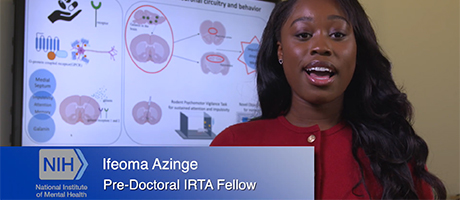 Ifeoma Azinge, Winner of the 2024 NIMH Three-Minute Talks Competition
-
Kathryn Altman, Winner of the 2024 NIMH Three-Minute Talks Competition